Reading time: about 22 minutes. Every formula is followed by its intuition, so you can skim the maths without losing the thread. The figures come from the original notebooks and are labelled in French.
Transparency note. This work was carried out on a personal basis, for learning purposes, with the help of an AI:
- for the code and the technical and methodological review;
- to understand the tools and the mathematical methods;
- for help with writing, translating and correcting the text;
- to generate the cover image of the post.
The choice of topic, the protocol, the checking of the results and the conclusions are mine, and so are any mistakes. How I use AI
This article distils my active research for week 37 (September 2026). I didn’t just read: I checked the sources, rewrote MinT from scratch, ran controlled experiments, reconciled the electricity demand forecasts of France’s 12 mainland regions, and tested a Bayesian reconciliation package. Everything is reproducible, with pinned versions, in the W37_hierarchical_reconciliation repository.
In short. Reconciliation guarantees coherence, not accuracy, and not calibration. I found four pieces of evidence:
- In theory: a bias in a single forecast contaminates all the others.
- Probabilistically: an interval advertised as 90 % at the total level can cover only 76 %.
- On real data: over 119 days of 2024, the simplest method (bottom-up) beats MinT.
- On retail sales: 98 % of the intervals reconciled by MinT start below zero.
1. The problem: forecasts that don’t add up#
Take a cooperative that sells in two French regions, each through two channels: supermarkets (GMS) and food service (RHD). That’s 7 series to forecast: the total, 2 regions and 4 region × channel pairs. Each series has its own model, tuned as well as possible. But nobody asked the models to agree with each other.
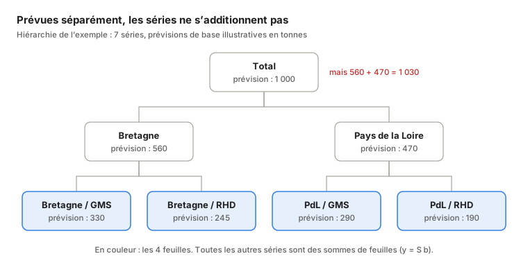
The structure is described by a summing matrix \(S\). The bottom series, the leaves \(b_t\), determine everything else:
$$ y_t = S\,b_t, \qquad S = \begin{pmatrix} 1 & 1 & 1 & 1\\ 1 & 1 & 0 & 0\\ 0 & 0 & 1 & 1\\ 1 & 0 & 0 & 0\\ 0 & 1 & 0 & 0\\ 0 & 0 & 1 & 0\\ 0 & 0 & 0 & 1 \end{pmatrix} \begin{matrix}\leftarrow \text{total}\\ \leftarrow \text{Bretagne}\\ \leftarrow \text{Pays de la Loire}\\ \leftarrow \text{Bretagne / GMS}\\ \leftarrow \text{Bretagne / RHD}\\ \leftarrow \text{PdL / GMS}\\ \leftarrow \text{PdL / RHD}\end{matrix} $$A forecast vector is coherent if it can be written \(S\,b\) for some \(b\): every sum adds up. Base forecasts \(\hat y\), produced series by series, almost never are.
The two classic answers throw information away:
- bottom-up sums the leaves and ignores the forecasts of the aggregates, which are often more stable;
- top-down splits the total using historical proportions and ignores what the leaf models know. If it computes those proportions on a history that includes the test period, it also leaks information from the future, and nothing in the metrics will flag it.
Optimal reconciliation sets out to use all the forecasts at once.
2. MinT in five minutes: reconciling is projecting#
The framework#
We look for a matrix \(G\) that maps the \(m\) base forecasts to \(n_b\) leaves, which are then summed back up:
$$ \tilde y = S\,G\,\hat y . $$Two conditions constrain the choice of \(G\):
| Condition | Formula | What it means |
|---|---|---|
| unbiasedness preservation | \(SGS = S\) | a vector that is already coherent is left unchanged |
| reconciled error variance | \(\operatorname{Var}(y - \tilde y) = S G W G^\top S^\top\) | with \(W = \operatorname{Var}(y - \hat y)\), the covariance of the base errors |
MinT (Minimum Trace, Wickramasuriya, Athanasopoulos and Hyndman, 2019) minimises the trace of that variance subject to \(SGS = S\). The solution has a closed form:
$$ G = \left(S^\top W^{-1} S\right)^{-1} S^\top W^{-1}, \qquad P = S\,G . $$The geometric intuition#
\(P\) is a projection (\(P^2 = P\)). Coherent vectors form a subspace of dimension \(n_b\) in \(\mathbb{R}^m\), and reconciling means bringing \(\hat y\) back onto that subspace. The whole question is: in which direction?
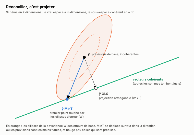
- OLS (\(W = I\)) projects orthogonally: every series is treated as equally reliable.
- MinT projects according to \(W^{-1}\). It picks the coherent point that is most plausible given the shape of the errors: it moves badly forecast series a lot and the others very little.
- Bottom-up is a projection too, with \(G = [\,0 \mid I\,]\): it only moves the aggregates.
| Method | Matrix \(W\) used | What it assumes |
|---|---|---|
| bottom-up | — (\(G = [0 \mid I]\)) | the aggregates add nothing |
| OLS | \(I\) | all errors are alike |
| WLS struct | \(\operatorname{diag}(S\mathbf{1})\) | variance proportional to the number of aggregated leaves |
| WLS var | \(\operatorname{diag}(\hat W)\) | individual variances, no correlations |
| MinT shrink | \(\lambda D + (1 - \lambda)\hat W\) | variances and correlations, regularised |
The detail that will matter later#
\(W\) is unknown. In practice it is estimated on the in-sample residuals of the base models, then regularised with Schäfer–Strimmer shrinkage: correlations are pulled towards zero with an intensity \(\lambda \in [0, 1]\) estimated from the data. Keep this in mind: it’s what makes MinT lose on real data (section 6).
3. What the 2026 literature says#
I read six papers, chosen to cover MinT’s blind spots. For each one, I checked what was claimed about it against its official abstract. The reading plan sometimes oversold them.

| Paper | What it brings | What the check corrected |
|---|---|---|
| Li, Chen, Taylor, Mao — A Forecast Combination Framework for Hierarchical and Grouped Time Series Reconciliation (2608.13886) | The optimal combination weights exactly recover MinT. Forty years of forecast-combination literature (shrinkage, penalties, positivity) become reusable. | — |
| Rønlev-Knudsen, Madsen, Møller — Online forecast reconciliation using linear models (2606.23326) | Reconciliation as a regularised regression, updated recursively: no need to re-estimate \(W\) at every run. | The case study is a temporal hierarchy, not a geographical one. Validate before transposing. |
| Nugteren, Abolghasemi, Mengersen, Drovandi — Hierarchical Bayes meets hierarchical forecasting (2606.23009) | A Bayesian model that targets the level where the decision is made. | Coherence is soft (penalised), not exact. |
| Wang, Johnson, Klee, Malloy — Billions-Scale Forecast Reconciliation (2602.05030) | Reconciliation over more than four billion values; least squares and share-based allocation coincide under conditions. | — |
| Panagiotelis, Gamakumara, Athanasopoulos, Hyndman — Probabilistic forecast reconciliation (EJOR, 2023) | The proper definition of reconciling a distribution, evaluated with the energy score and the variogram score. | — |
| Biswas, Zambon, Nespoli, Corani — Nonlinear Probabilistic Forecast Reconciliation (2604.26668) | What happens when \(y = Sb\) no longer holds: logs, ratios, average prices. | — |
The check was limited to abstracts and official pages, not the full PDFs.
Three trends stand out:
- Reconciliation is becoming an estimator, not a post-processing step. Seen as forecast combination or as regularised regression, it can be regularised, tested and defended in an architecture review.
- The scale objections are gone. Four billion values on one side, recursive estimation on the other.
- The open front is probabilistic and nonlinear reconciliation. That is exactly where point-forecast MinT has nothing left to say. Section 5 shows it.
4. Rewriting MinT yourself#
Calling MinTrace(method="mint_shrink") takes one line. But until you have written the formula
yourself, you can’t explain a strange result. So I reimplemented MinT shrink in NumPy, and I
didn’t allow myself to read the HierarchicalForecast
code until mine was frozen. Here is the core, condensed:
import numpy as np

def mint_shrink(E, S):
    """E: in-sample residuals (T × m), S: summing matrix (m × nb). Returns P = SG."""
    T, m = E.shape
    W1 = E.T @ E / T                          # sample covariance
    Z = E / np.sqrt(np.diag(W1))              # standardised residuals
    R = Z.T @ Z / T                           # correlations
    w = Z[:, :, None] * Z[:, None, :]         # T × m × m: naive, see below
    var_r = T / (T - 1) ** 3 * ((w - R) ** 2).sum(axis=0)
    off = ~np.eye(m, dtype=bool)
    lam = np.clip(var_r[off].sum() / (R[off] ** 2).sum(), 0, 1)   # Schäfer–Strimmer λ
    W = lam * np.diag(np.diag(W1)) + (1 - lam) * W1
    WiS = np.linalg.solve(W, S)                       # W⁻¹S, without inverting W
    G = np.linalg.solve(S.T @ WiS, WiS.T)             # (S'W⁻¹S)⁻¹ S'W⁻¹
    return S @ G
On a synthetic hierarchy (2 regions × 2 channels, 80 quarters, AutoETS models), the checks
pass:
| Check | Threshold | Measured |
|---|---|---|
| \(P^2 = P\) and \(SGS = S\) | < 1e-12 | 2.2e-16 |
| incoherence of the reconciled forecasts | machine precision | 5.7e-14 |
| relative gap to HierarchicalForecast 1.5.1 | < 1e-3 | 1.07e-5 |
| non-zero gap | > 0 | yes |
The last check is deliberate: an exactly zero gap would have meant I had copied their code. That small residual gap taught me three things.
Lesson 1: one method name covers several estimators#
The research plan put the gap down to a difference in how \(\lambda\) is computed. That’s wrong:
the two \(\lambda\) values agree to within 2e-5. About 99.8 % of the gap comes from the base
covariance. The library centres the residuals and divides by \(T - 1\) (np.cov), whereas my
version uses \(E^\top E / T\). With the same convention, the gap drops to 3e-6.
The practical consequence: mint_shrink covers at least three implementation choices (centring,
ddof, the \(\lambda\) variant) that change the published number. If two teams compare their runs,
they need to pin the version and document the estimator.
Lesson 2: shrinkage is a condition for existence#
Even with 72 observations for 6 series, the sample covariance is ill-conditioned (condition number ≈ 3·10⁴). An aggregate’s residual is almost the sum of its leaves’ residuals, so the columns of \(E\) are nearly collinear. Shrinkage brings the condition number down to ≈ 23.
With more series than observations (\(m > T\)), it gets worse: \(\hat W\) has rank \(T\), so it is singular. With \(T = 4\) and \(m = 6\), its condition number reaches 1.7·10¹⁷. Shrinkage then picks \(\lambda = 0.907\) on its own and brings the condition number down to 10. Shrinkage is not a convenience: without it, MinT doesn’t exist on a real catalogue. 40,000 products over three years of weekly history means \(m/T \approx 250\).
Lesson 3: the wall is also a memory wall#
The line marked “naive” builds a \(T \times m \times m\) tensor: 31 GB for 5,000 series. My first version got the Jupyter kernel killed by the operating system. Yet \(\lambda\) only depends on off-diagonal sums, which can be computed from the \(T \times T\) Gram matrix. Memory goes from \(O(T m^2)\) to \(O(T^2 + Tm)\), i.e. 0.6 GB, for a result identical to within 1e-10. Beyond that, it’s \(W\) itself that must no longer be formed. A diagonal plus a rank-\(T\) matrix can be inverted with the Woodbury identity, without ever building an \(m \times m\) matrix.
5. Three places where MinT breaks#
MinT is optimal under assumptions: unbiased base forecasts, known \(W\), linear constraints, continuous quantities. I set up a controlled experiment for each of these assumptions. Each time, I looked for the point where it gives way.
5.1 MinT spreads bias#
The condition \(SGS = S\) preserves unbiasedness; it doesn’t create it. The counter-example fits in four series: one total and three leaves. The forecasts are exact everywhere except for a +15 bias on the total. \(W\) trusts the total 9 times more than each leaf.
| Series | Truth | Base | Bottom-up | MinT | MinT error |
|---|---|---|---|---|---|
| Total | 60 | 75 | 60 | 74.46 | 14.46 |
| Leaf 1 | 10 | 10 | 10 | 14.82 | 4.82 |
| Leaf 2 | 20 | 20 | 20 | 24.82 | 4.82 |
| Leaf 3 | 30 | 30 | 30 | 34.82 | 4.82 |
Bottom-up ignores the total and sees nothing. MinT, which trusts it, injects the bias into every leaf. Because reconciliation is linear, the reconciled bias equals \(P \times\) the base bias: it spreads along a column of \(P\).
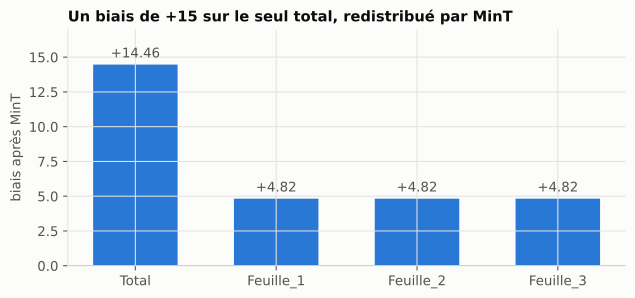
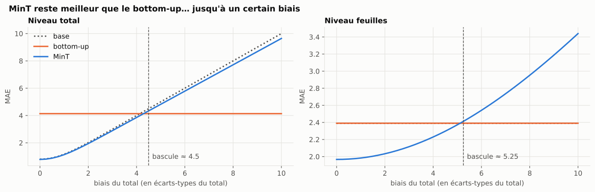
It isn’t all or nothing: there is a threshold. In simulation (20,000 draws), MinT stays ahead of bottom-up as long as the bias on the total is below ≈ 4.5. Above that, it becomes worse at the total; above ≈ 5.25, it is also worse at the leaves, i.e. at every level.
5.2 MinT reconciles means, not quantiles#
This is the heart of the week. An inventory manager doesn’t decide on a mean. They decide on a quantile: the stock that covers demand 90 % of the time. And the quantile of a sum is not the sum of the quantiles.
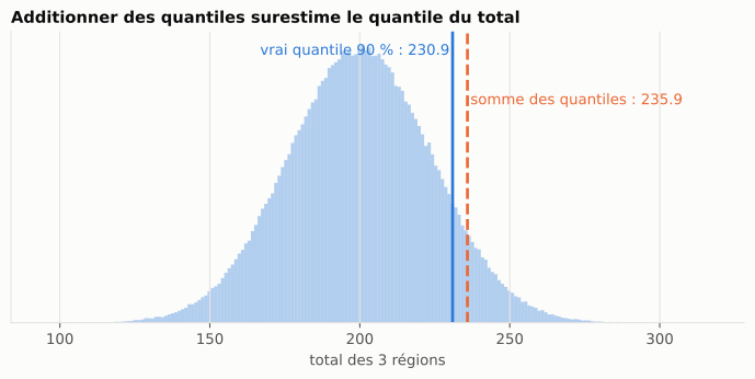
Consequence: no vector of quantiles is coherent. Coherence is a property of the joint distribution, not of the marginals.
The experiment is fully simulated, so the truth is known: one total and three Gaussian regions, correlated at \(\rho = 0.6\) (the weather moves them together). Each base model is perfect on its own series. The means are already coherent, so everything we observe is a pure “quantile” effect. We compare three ways of getting reconciled 90 % quantiles:
- A. Apply \(P\) directly to the quantiles. This is the most common mistake.
- B. Draw samples from each series independently, project each sample, then read off the quantiles.
- C. The same, but with joint samples that respect the dependence between series.
| Series | Coverage A | Coverage B | Coverage C |
|---|---|---|---|
| Total | 0.922 | 0.764 | 0.900 |
| Region 1 | 0.887 | 0.878 | 0.900 |
| Region 2 | 0.890 | 0.888 | 0.899 |
| Region 3 | 0.893 | 0.894 | 0.901 |
Target: 0.900. 400,000 draws, fixed seed.
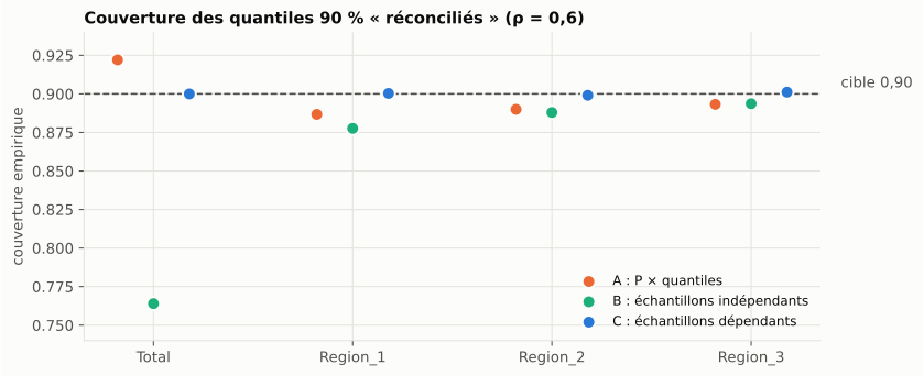
How to read this table:
- A is wrong in both directions at once. It over-covers at the total and under-covers in the regions. No global factor can fix it. The resulting vector adds up perfectly, but it isn’t the quantile of anything.
- B, which looks rigorous, is the worst: 76 % coverage at the total for 90 % advertised. Projecting samples is the right mechanism. But independent draws erase the dependence, and the variance of the sum is massively underestimated.
- C is calibrated everywhere. Its only difference from B is the dependence structure.
Sweeping the correlation makes the result hard to dispute:
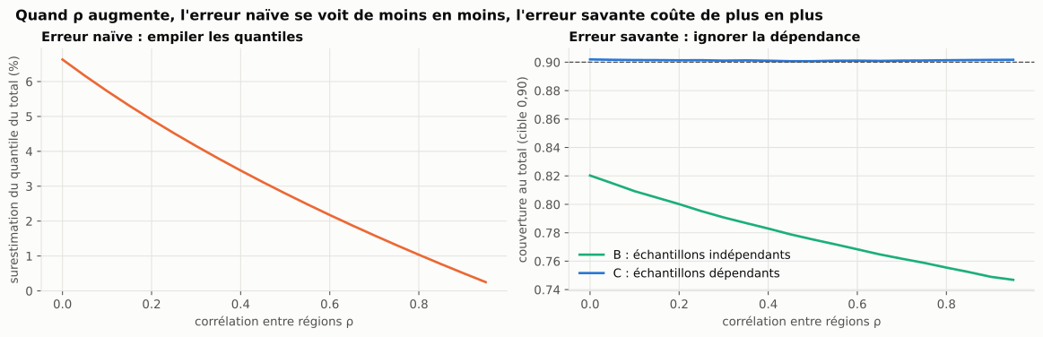
| \(\rho\) | Gap “sum of q90s” / “q90 of the sum” | Coverage B at the total |
|---|---|---|
| 0.0 | +6.6 % | 0.816 |
| 0.3 | +4.2 % | 0.787 |
| 0.6 | +2.2 % | 0.764 |
| 0.9 | +0.5 % | 0.746 |
In practice, the true covariance is unknown. The solution is a joint bootstrap of the in-sample
residuals: we resample time points, and all series are drawn at the same time point. This gets
back to 0.902 at the total. A series-by-series bootstrap reproduces B’s error (0.760). In
HierarchicalForecast, these are the Bootstrap and PERMBU methods.
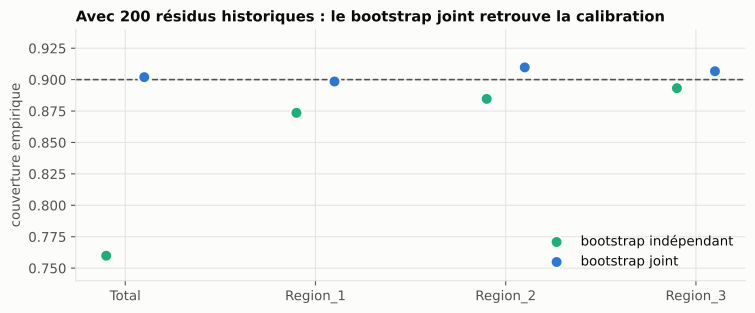
A simple rule follows: same time point, all series. A bootstrap that draws residuals at different dates for different series (histories of unequal length, gaps) is method B in disguise.
5.3 MinT doesn’t know about zero#
The third implicit assumption: quantities are continuous and symmetric. On slow-moving product sales (often 0, sometimes a spike), a Gaussian with the right variance spills well below zero.
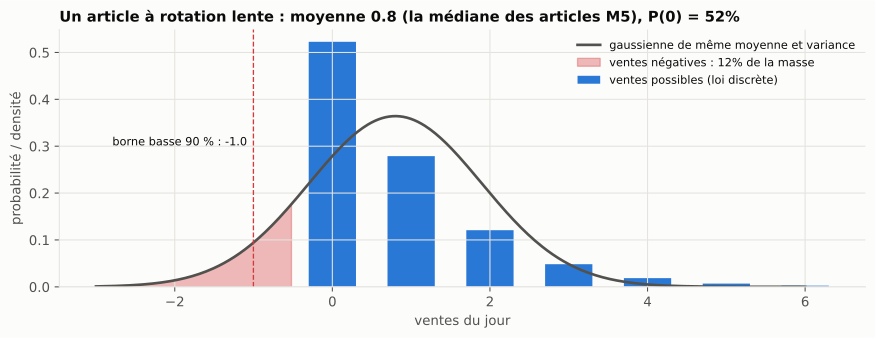
I measured it on one store from the M5 dataset (Walmart, store CA_1: 3,049 products and 11 aggregates, one-day-ahead forecast), comparing Gaussian MinT with BayesReconPy. This package doesn’t project: it conditions. It keeps the joint distribution of the products on the non-negative integers and reweights it by what the aggregate forecasts say (Bayes’ rule).
| Gaussian MinT | bottom-up | MixCond | TD-cond | |
|---|---|---|---|---|
| products with a negative mean | 11 | 0 | 0 | 0 |
| products whose 90 % lower bound is < 0 | 2,992 (98 %) | 0 | 0 | 0 |
| product RPS (lower = better) | 0.819 | 0.676 | 0.674 | 0.669 |
| aggregate MIS (lower = better) | 1,825 | 2,330 | 2,312 | 444 |
The number that matters depends on the decision. For a decision based on the mean, 0.36 % of the forecasts are negative. For a service level, it’s 98 %. The mechanism is easy to read: with a diagonal \(W\), each product’s adjustment is proportional to its variance. The “almost always 0, sometimes a big spike” products therefore absorb most of the correction and go below zero.
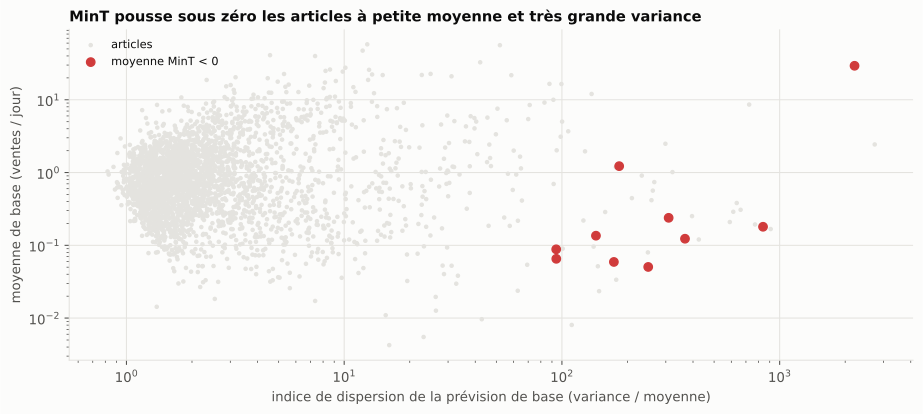
Two more observations:
- Bottom-up and MixCond make the aggregate intervals five times worse. Assuming 3,049 independent products gives a total that is far too narrow: it’s method B from the previous section, at scale. TD-cond, which starts from the aggregates, avoids that trap and stays the most accurate at both levels.
- My numbers reproduce the official R vignette of the
bayesReconpackage on the same store, with a median gap of 0.15 skill-score points.
pulp<4). Its licence is
contradictory: MIT in the metadata, LGPL-3.0 in the repository. Finally, reconc_td_cond modifies
its inputs in place. It’s an excellent specialised tool, but you need to know its conditions of
use.6. On real data: twelve regions, one France#
The previous experiments are controlled. The next step was to confront MinT with real data. I used the electricity demand of France’s 12 mainland regions (éCO2mix, RTE, via ODRÉ, Licence Ouverte v2.0). The business goal: deliver hourly day-ahead forecasts where the sum of the regions exactly matches the national total.
Check the data before forecasting#
Three findings came before the first forecast:
- Nouvelle-Aquitaine stops at the end of 2024, while the other regions continue. Since 2025, the sum of the regions is no longer the national total. The protocol is therefore limited to 2013–2024.
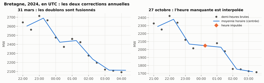
- The source has a daylight-saving defect, every year and in every region: two duplicates at
the end of March, one missing hour at the end of October. A missing row distorts a total
without raising any error, which is more dangerous than a
NaN. - The official total isn’t always the sum of the regions. The gap exceeds 200 MW in October 2016. A year-by-year test shows it stays below 6 MW (rounding) from 2014 to 2024, except 2016: over the period actually used, reconciling towards that total makes sense.
The protocol, fixed before seeing the results#
- Hourly step: mean of the half-hours, in UTC. MW stay MW, and no day has 23 or 25 hours.
- Base models:
SeasonalNaive(168)as the floor,MSTLwith double seasonality (24 h and 168 h) as the reconciled model. - Window: rolling 52 weeks, strictly prior to each origin.
- Methods compared: bottom-up, OLS, WLS struct, WLS var, MinT shrink.
- Metric: MASE per level (France, then the average over regions), never a global average.
The original plan called for 4 origins: four Tuesdays in November 2024. I added a robustness study over 119 origins, one every three days across 2024.
The ranking flips#
Coherence is guaranteed: the maximum incoherence is exactly 0 MW after reconciliation, versus 672 MW for the base forecasts. But accuracy tells a different story depending on the number of origins:
| Mean MASE, 119 origins | France | Regions |
|---|---|---|
| SeasonalNaive (floor) | 0.947 | 0.939 |
| bottom-up | 0.352 | 0.427 |
| WLS var | 0.356 | 0.430 |
| WLS struct | 0.358 | 0.432 |
| OLS | 0.366 | 0.439 |
| MinT shrink | 0.370 | 0.439 |
Over 4 origins, MinT seemed to win at the regional level (−2.2 %), without significance. Over 119 origins, bottom-up is the best method at both levels, and MinT shrink does worse than it on all 13 series, without exception. The four Tuesdays had landed on the favourable side of a very wide distribution. After Holm correction, the evidence is moderate (p ≈ 0.05), but the sign is consistent. Four origins are not enough to rank methods.
The cause: a hidden assumption in mint_shrink#
MinT assumes that the estimated covariance \(W\) resembles that of the true forecast errors. I tested that assumption directly. MSTL’s in-sample residuals are smoothing leftovers, correlated at 0.11 on average between regions. The true out-of-sample errors are correlated at 0.56 (bootstrap interval [0.45; 0.65]). MinT is therefore reconciling with the wrong map of the errors.
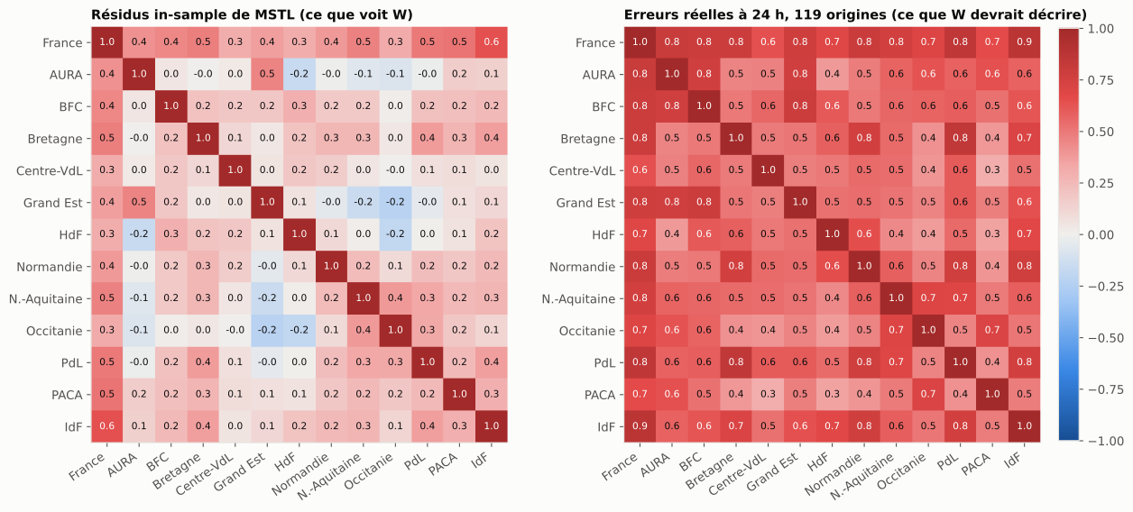
To isolate the cause, I ran a controlled experiment. Everything stays the same except \(W\), which I estimate on the out-of-sample errors of past origins, so still without leakage.
| 99 origins | Regional MASE vs bottom-up | p (Wilcoxon) |
|---|---|---|
| MinT shrink, in-sample \(W\) | +2.6 % | 0.017 |
| MinT, \(W\) estimated on past errors | −0.1 % | 0.83 |
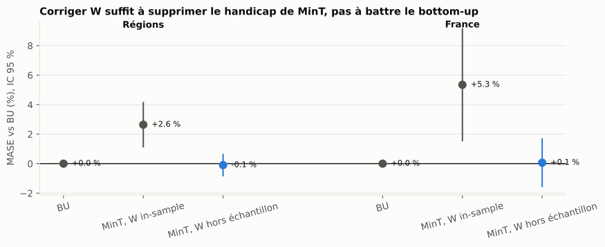
Fixing \(W\) removes the handicap, but doesn’t make MinT win. That’s plausible: regional errors are strongly correlated and share the same sign (a cold snap hits everyone), so there is no cross-sectional information to exploit.
My recommendation for this case:
- Ship bottom-up. It meets the goal (exact coherence), it’s the most accurate here, and it can be explained in one sentence: “the national figure is the sum of the regions”.
- Don’t use
mint_shrinkwith the in-sample residuals of a smoothing model. If MinT is needed, estimate \(W\) on rolling backtest errors. - Invest in the base models (temperature, public holidays). The largest errors are shared by all regions, and no reconciliation can recover them.
7. In production: where does reconciliation live?#
One last question, about architecture: should reconciliation be a batch job, a step inside the API, an SQL view or an estimator updated online? I chose a materialised batch job with a blocking quality gate. The reasons fit in one diagram:
flowchart TD
    H[History and covariates] --> B["1. Base forecasts
one model per series → incoherent ŷ"]
    B -->|ŷ + training residuals| R["2. Reconciliation
P = S(S'W⁻¹S)⁻¹S'W⁻¹"]
    S["Versioned S + fingerprint"] --> R
    R --> Q(["3. Quality gate
coherence · negatives · MASE per level"])
    Q -->|fail| X[Publication blocked + alert]
    Q -->|pass| T[("forecast_reconciled table
immutable artefact: run_id, S fingerprint, W version")]
    T --> A["API /forecast?level=
read-only"]
The non-negotiable point: the API never reconciles on the fly. Otherwise two simultaneous calls on two levels can return numbers that don’t add up, which is exactly the problem we set out to remove. Coherence is a property of the artefact, not of the request.
| Option | For | Against | |
|---|---|---|---|
| Materialised batch | coherent by construction, auditable | refresh latency | ✅ chosen |
| On the fly in the API | always up to date | coherence not guaranteed across calls | ❌ |
| SQL view | zero infrastructure | MinT in SQL is unmanageable, you end up with bottom-up in disguise | ❌ |
| Recursive online estimation | \(W\) tracks regime changes | mutable state to version and replay | ⏳ later |
Writing this contract as executable code, with tests where each rule fails, corrected four things in the paper version:
- Fallback to a simpler method must not trigger when \(m > T\). That is precisely the case shrinkage exists for (lesson 2). It triggers on the measured condition number of \(W\).
- An absolute coherence tolerance doesn’t mean the same thing at 10 MW and at 50 GW. I added a relative tolerance.
- The “no MASE degradation” rule applies level by level, never on average. Otherwise a gain at the national level hides a loss at the decision level.
- The fingerprint of \(S\) also covers the labels. A renamed leaf changes the hierarchy without changing the matrix.
reconciler:
  method: mint_shrink
  fallback: wls_struct          # triggered by measured cond(W), not by m > T
  covariance_window: 104        # weeks, strictly prior to the origin
quality_gate:
  coherence_tol_abs: 1e-6
  coherence_tol_rel: 1e-9       # floating-point noise grows with the values
  max_negative_share: 0.001     # Gaussian MinT on M5: 0.0036 → blocked
  compare_to_baseline: bottom_up  # fail if MASE degrades by more than 2 % at ANY level
  fail_action: block_publish
8. What I take away#
- Reconciliation sells coherence, not accuracy. Accuracy gains are frequent, never guaranteed, and they depend on assumptions you can test.
- Always compare with bottom-up, level by level. Beating incoherent forecasts proves nothing, and a global average hides the level where the decision is made.
- \(W\) is the weak link. Estimated on in-sample residuals, it can describe errors that don’t exist. Shrinkage is essential, but it doesn’t fix a bad source.
- Never reconcile quantiles. Reconciling a distribution means projecting joint samples. Independent draws give a 90 % interval that covers 76 %.
- Counts need different tools. A Gaussian has no business near zero. Conditioning (TD-cond) is coherent, non-negative and more accurate, all at once.
- Check before you believe: the data (daylight saving, a missing region), the sources (what the abstract actually says), the packages (installation, licence) and the rankings (4 origins versus 119).
What’s next. Everything above collapses if \(W\) is estimated on contaminated residuals, if the hierarchy changes without notice, or if a leaf has a gap. So week 38’s research is about building leak-free temporal features: correct rolling windows, point-in-time data, reference tables that change over time. The common thread: it’s not the model that leaks, it’s the join.
Reproduce and go further#
The code, the 14 notebooks and the 88 tests are in the
gwils28/W37_hierarchical_reconciliation
repository (Python 3.12, HierarchicalForecast 1.5.1, statsforecast 2.1.1, BayesReconPy 0.5.0,
versions locked with uv). Every number in this article comes from a uv run w37 … command. The
repository is in French.
Sources
- Wickramasuriya, Athanasopoulos, Hyndman, Optimal forecast reconciliation for hierarchical and grouped time series through trace minimization, JASA, 2019.
- Li, Chen, Taylor, Mao, A Forecast Combination Framework for Hierarchical and Grouped Time Series Reconciliation, arXiv, 2026.
- Rønlev-Knudsen, Madsen, Møller, Online forecast reconciliation using linear models, arXiv, 2026.
- Nugteren, Abolghasemi, Mengersen, Drovandi, Hierarchical Bayes meets hierarchical forecasting, arXiv, 2026.
- Wang, Johnson, Klee, Malloy, Billions-Scale Forecast Reconciliation, arXiv, 2026.
- Panagiotelis, Gamakumara, Athanasopoulos, Hyndman, Probabilistic forecast reconciliation: properties, evaluation and score optimisation, EJOR 306(2), 2023.
- Biswas, Zambon, Nespoli, Corani, Nonlinear Probabilistic Forecast Reconciliation, arXiv, 2026.
- Schäfer, Strimmer, A shrinkage approach to large-scale covariance matrix estimation, SAGMB, 2005.
- Biswas et al., BayesReconPy, JOSS 10(111), 2025.
- Living bibliography: awesome-forecast-reconciliation.
- Data: regional éCO2mix, Open Data Réseaux Énergies (ODRÉ), RTE, Licence Ouverte v2.0; M5 Forecasting.