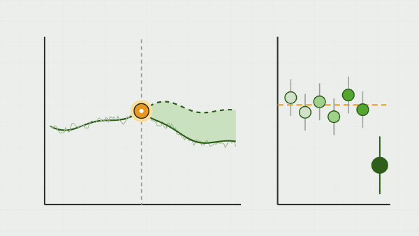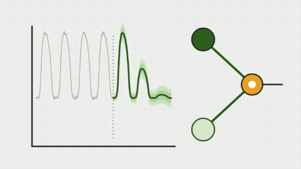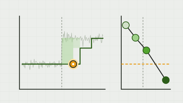
2.4%
of promotion jumps measurable
onpromotion, by a rule fixed before the results0.83 to 0.90
95% coverage on planted truth
64%
of the promotion budget unspent
Transparency note. This work was carried out on a personal basis, for learning purposes, with the help of an AI:
- for the code and the technical and methodological review;
- to understand the tools and the mathematical methods;
- for help with writing, translating and correcting the text;
- to generate the cover image of this page.
The choice of topic, the protocol, the checking of the results and the conclusions are mine, and so are any mistakes. How I use AI
This repository applies the post
Causal impact in time series: the counterfactual and its placebos
to a client brief. The causal_ts package from the tech watch (counterfactual, placebos,
isolation, baselines) is reused as a pinned dependency; everything specific to promotions is
new. The repository, its notebooks and its figures are in French.
The goal#
NovaRetail is a fictional grocery chain that runs promotion after promotion without knowing their incrementality. Management’s suspicion: a large share of the sales “on promotion” would have happened anyway, with pull-forward (the dip after the promotion) and cannibalisation between families on top. The brief asked for a counterfactual per campaign, an uplift with an interval, an elasticity curve per family, placebo backtesting, an orchestrated stack and monitoring.
The data is the Kaggle Store Sales competition (Corporación Favorita, Ecuador): 54 stores, 33 families, 1,684 days, a count of items on promotion per day and family, the oil price, holidays, and the earthquake of 16 April 2016 as an exogenous shock.
What I wanted to learn came down to three questions:
- what becomes of a design validated on clean panels when the treatment is not defined, zeros have several meanings and the controls cannibalise each other;
- how to score an estimator on real series, with no known truth, other than by looking at the width of its intervals;
- what a pipeline and monitoring can watch over a quantity nobody ever observes, a counterfactual.
The approach#
The work follows six blocks, one folder each, with a results README per block. The code lives
in one package (src/novaretail), a CLI nr chains the steps and writes its summaries to
data/results/*.json, and the seven notebooks call the package with no logic of their own. The
brief and the framing decisions are in plan.md, and the protocol (credibility thresholds,
reference model, planted truth) was fixed there before the first result. The working method is
the one in
Claude Code for data science: what changes in my working method.
- 1
Data
A dense panel, five kinds of structural zeros (store not open yet, family never sold, closure, family not listed yet, long zero run) set toNaNrather than imputed, a calendar with transferred holidays, paydays and the oil gradient, and a synthetic Favorita-like world with a known counterfactual to build the whole chain before the Kaggle files. - 2
Identification
The treatment is constructed: a campaign is a jump ofonpromotionabove its rolling median, for at least three days, preceded by 120 quiet days. The control pool is a registry of rules (declared substitution edges, no promotion in the window, not the same city), never a choice by fit. Then donor isolation by placebo in space. - 3
Estimation
Thecausal_tslocal-level counterfactual per campaign, effects in units read path by path and split into during, after and net; synthetic control, augmented synthetic control, DiD and OLS on the same interface; Double ML for the response to intensity; the earthquake as a test bench. - 4
Backtesting
Truth planted in the real series: effects of 0, 5, 15 and 30%, step, ramp and pulse shapes, with or without pull-forward and cannibalisation. Each estimator is scored by its coverage, its false positives at zero effect and its power, not by its width. - 5
Pipeline
Local Dagster assets (panel, campaigns, estimates, backtest, monitoring, calendar), MLflow as a registry of estimates and their checks, a sha256 manifest of the raw files instead of DVC. No Docker, no cloud. - 6
Monitoring and calendar
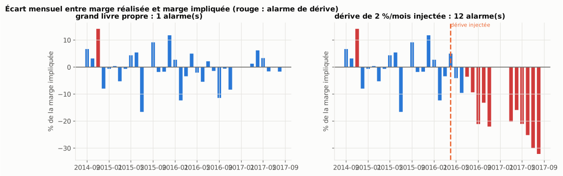
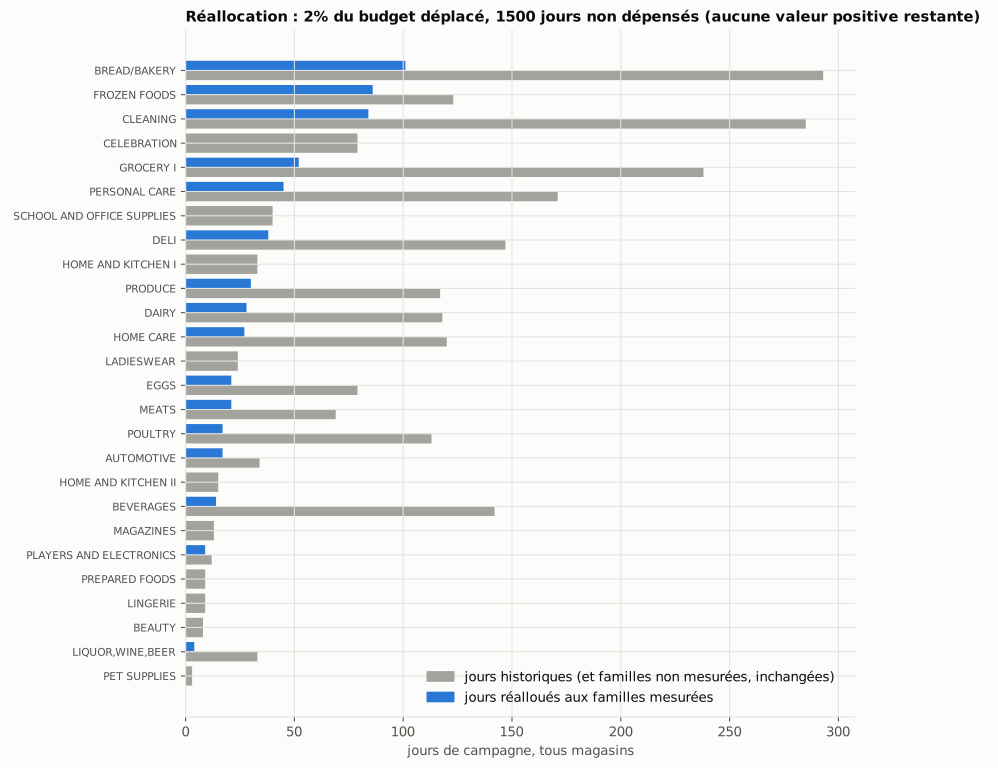
Four signals (pre-period fit, rolling placebo, isolation, donor-target stability), a margin reconciliation on a simulated ledger, and a calendar reallocation at constant budget on the lower bound of the intervals.
What the files corrected in the brief#
The brief described a different dataset and a different question from what the files allow. Each gap was settled on the data, then written down.
| The brief says | What the data says |
|---|---|
| “Favorita omits the zeros, decide whether to rebuild them” | The file is dense (one row per store, family and day, except Christmas Day). The job is the opposite: sorting zeros that are there. 31% of rows are zero, and 80% of those zeros are structural. |
| “Price elasticity curve per family” | No price in Favorita; onpromotion counts items. The deliverable becomes a response to promotion intensity by Double ML, and is named as such. |
“Treatment: onpromotion > 0” | Most families are promoted permanently at a low level. A campaign is a jump above the background, and the share of promoted days measurable by this design is the first result. |
| “Non-promoted families of the same store as controls” | That is the case the tech watch showed to be biased (+26% with a cannibalised donor, placebo in time green). The pool is a registry, then an isolation. |
| “Credible interval” | Frequentist prediction intervals, scored by their coverage measured on truth planted in the real panel. |
| “Earthquake: perfect exogenous shock” | A test bench for the method, not a promotion. The donors sold more themselves; the effect is a lower bound. |
| “Predicted uplift against realised margin” | No margin in Favorita. The reconciliation is shown on a simulated ledger with an injected drift. |
The results#
Every number comes from data/results/*.json, produced by the CLI on the Kaggle files.
How many promotions are measurable#
Out of 67,458 jumps in onpromotion, the detection rule keeps 1,592. The rest is too short
(the noise of an item count), falls in a pre-period already taken by another campaign, or
overlaps a structural zero. The kept campaigns last 3 to 20 days (deciles), 6 at the median. On
a stratified sample of 301 estimated campaigns, 170 pass the credibility protocol (pre-period
R², one-step coverage, Ljung-Box, placebo in time, donor isolation), 114 fail and 17 have too
few donors.
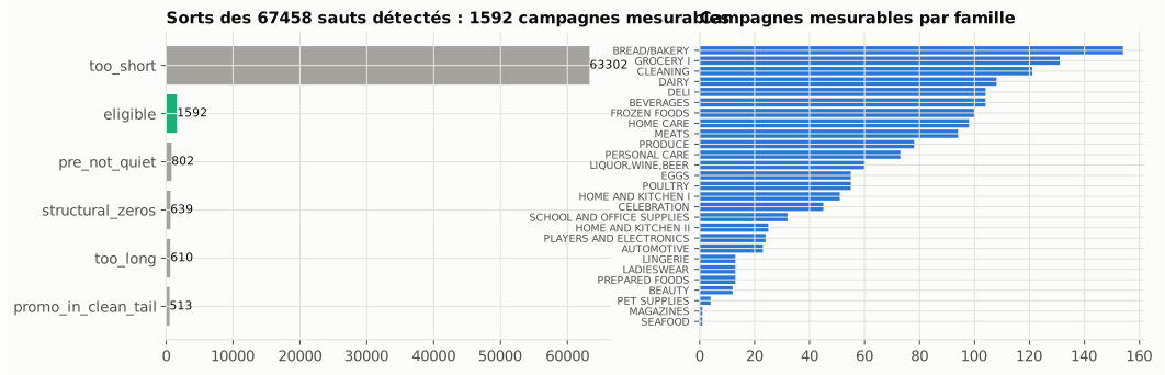
onpromotion: 1,592 measurable campaigns, 63,302 jumps too short. Right, measurable campaigns per family: ten families out of 33 have none.What a campaign is worth#
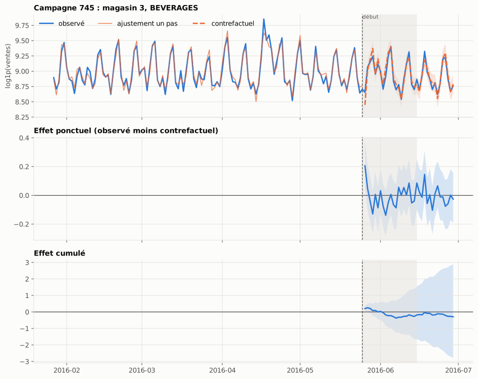
Over the 170 credible campaigns, the median lift during the campaign is +1.2%, with deciles at −8% and +13%. 7% of campaigns have a positive lower bound during the campaign, 5% on the net (campaign plus 14 days); 1 to 2% have a negative upper bound. The net sum over the 170 campaigns is −0.6% of the counterfactual. Pull-forward is not measurable at this level: the median share of units taken back after the campaign is −14%, a slight surplus rather than a dip, with intervals that contain zero almost everywhere.
What the design is worth#
This is the part that matters. On quiet windows of real series, with the real donor registry, a known effect is written into the series, and each estimator is scored on the cumulative effect.
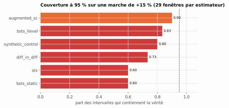
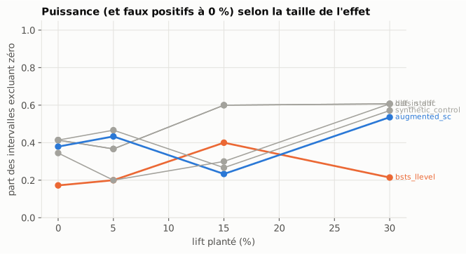
| Estimator | 95% coverage (15% step) | False positives at zero effect | Power at +5% / +15% |
|---|---|---|---|
| BSTS local level | 0.83 | 17% | 20% / 40% |
| Augmented synthetic control | 0.90 | 38% | 43% / 23% |
| OLS and static BSTS | 0.60 | 41% | 37% / 60% |
| Synthetic control | 0.80 | 41% | 47% / 27% |
| Difference in differences | 0.73 | 34% | 20% / 30% |
Three readings:
- Nobody reaches 95% on real series. The tech watch measured 0.92 to 0.94 for the local level on synthetic panels; here 0.83 to 0.90 depending on the specification. The iid-error estimators sit at 0.5 to 0.7 and fire on nothing four times out of ten.
- The 17% false positive rate is the reference for the placebos. With eight fake dates, 1.4 firings are expected on nothing; the protocol threshold (at most 2 out of 8) therefore rejects a quarter of campaigns by construction, and that is intended.
- Power is low. A 5% lift over seven days is detected two times out of ten, barely above the false positive rate; 15%, four times out of ten. This design cannot measure a small promotion on a single store-family series.
The earthquake, as a test bench#
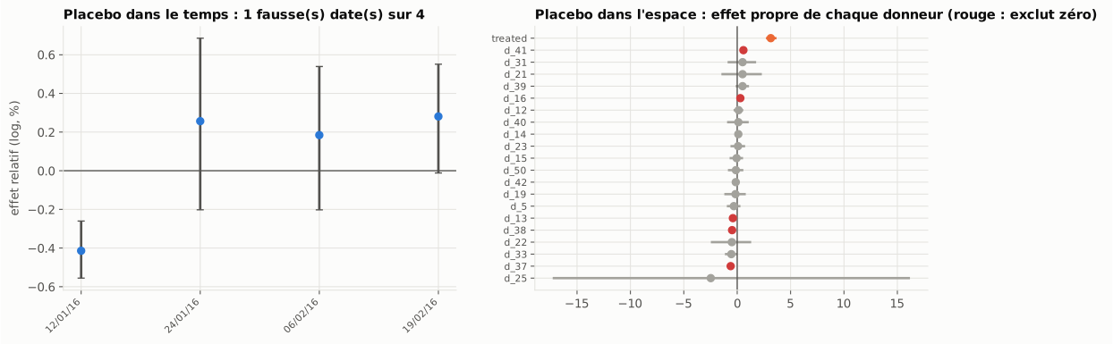
The stores of the stricken provinces (Manabí, Esmeraldas) against twenty stores of distant provinces: +39% in units over eight weeks [+32%; +46%], or 572,000 units, with an effect that grows from +10% in the first week to +45 to +55% through the eighth. The placebo in space shows that 5 donors out of 20 have an own effect that excludes zero: emergency relief purchases made the whole country sell more. The effect on the stricken provinces is therefore a lower bound, and the interference is visible because we know where to look.
The response to intensity, and why it does not feed the calendar#
Double ML gives a pooled θ of 0.15 to 0.59 depending on what the nuisances contain (lags,
months, trend), with tiny standard errors. Holdout 0.36 against 0.34 in training, DoubleML 0.38
as a cross-check, a monotone dose-response by bins. The concordance with the lifts of the 170
measured campaigns is nil (correlation 0.02). The instability is the result: a promotion’s date
is not “as good as random” given calendar controls, and DML does not fix that. PRODUCE’s θ (5)
comes from an onpromotion that is about 200 one day a week and 0 or 1 on the others: a
recording regime, not a response.
Monitoring and calendar#
The rolling placebo on never-treated windows exceeds 10% false positives over two thirds of the period: the design is on permanent alert, and that is the right information. With 17% false positives per donor and twelve donors, isolation removes two by noise on 114 campaigns; donor by donor coefficients change sign 223 times between two campaigns of the same target. Signals 3 and 4 are only readable once signal 2 is back under 10%.
The calendar reallocates campaign days per store, at constant budget, towards the families with the highest value per day on the lower bound. Over 2,327 days and 53 stores, 48 days move (2%) and 1,500 are left unspent (64%): no measured family in the store has a positive value on the lower bound. Ten families out of 33 never have a measurable campaign.
What got in the way#
- The treatment was the problem, not the estimator.
onpromotionis a count with a permanent background, a weekly spike on PRODUCE and recording regimes that change in 2016. Half the project’s time went into deciding what a zero is and what a campaign is. The choice between BSTS and synthetic control, for its part, is settled by coverage. - The brief described a different file. The 2017 version of the Favorita dataset omits zero sales; the 2021 version is dense. Three more kinds of structural zeros than planned showed up at load time: 595 of the 1,729 store-family series start more than 30 days after the store opens, PRODUCE has whole quarters at zero in 2014 and 2015, and long zero runs are not intermittency.
- Simulated paths sometimes diverge. On the
log1pscale, a path that runs away weighs millions of units once transformed back. Divergent paths are dropped, counted and checked; a campaign with more than 5% of them is not credible by protocol. - Real series cost ten points of coverage. Zeros, extreme values, regime changes: the difference between a clean panel and a file. The RMSE of some estimators comes from a few windows where a donor jumps and a model without a stochastic level extrapolates that jump.
- Study sizes. 30 windows per backtesting cell, or ±0.1 on each coverage; 300 campaigns estimated out of 1,592 (13 minutes), a single draw of the stratification. The orders of magnitude are stable from one run to the next, the second decimal is not.
What I take away#
- Management’s suspicion holds, but the evidence is weak: the net sum of the 170 credible campaigns is zero to −0.6%, and the same design detects a 5% lift planted in these series only once in five. “No measurable effect” and “no effect” are two different sentences.
- A counterfactual is a forecast, and its causal content rests on the design: which campaigns, which donors, which placebos. That design is scored on known truth before producing a number, and the score on real series is lower than on synthetic panels.
- The control pool is declared, not fitted: the best fit is often the closest substitute.
- The DML θ are not elasticities, and their sensitivity to the specification says the identification assumption does not hold on this panel. They are reported for that reason.
- What the method cannot see, nothing here can see: a donor-target relationship that breaks on the campaign date. Only a reconciliation with realised margin or a real holdout settles it. The recommendation to NovaRetail is to measure fewer campaigns and anchor a few of them by experiment, with randomly drawn control stores.
Reproduce#
git clone https://github.com/gwils28/novaretail-promo-incrementality
cd novaretail-promo-incrementality
make install                      # uv sync (Python 3.13), causal_ts as a pinned git dependency
make test-fast                    # unit tests on the synthetic world
# drop store-sales-time-series-forecasting.zip (Kaggle) in data/raw/, then:
uv run nr ingest && uv run nr campaigns
uv run nr estimate --param-draws 40          # registry, counterfactual, placebos, isolation, verdict
uv run nr backtest --n 30                    # planted truth, scores per estimator (2 min)
uv run nr quake && uv run nr dml             # earthquake (15 s), response to intensity (3 min)
uv run nr monitor && uv run nr calendar      # signals, simulated reconciliation, reallocation
make notebooks                               # re-executes the seven notebooks (10 min)
Without the Kaggle files, uv run nr ingest --source synthetic runs the same chain on the
synthetic world. Data: Corporación Favorita, Kaggle competition Store Sales - Time Series
Forecasting.