| model | mase | smape | wape | cov80 | cov90 | width90 | winkler90 | sql |
|---|---|---|---|---|---|---|---|---|
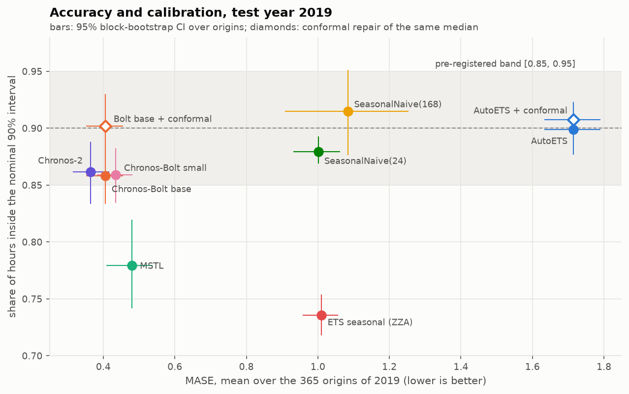
| SeasonalNaive(24) | 1.001 | 0.03 | 0.059 | 0.824 | 0.879 | 0.293 | 7.079 | 0.429 |
| SeasonalNaive(168) | 1.084 | 0.03 | 0.061 | 0.854 | 0.915 | 0.33 | 6.917 | 0.448 |
| AutoETS | 1.715 | 0.053 | 0.102 | 0.772 | 0.899 | 0.45 | 8.742 | 0.669 |
| AutoETS + conformal | 1.715 | 0.053 | 0.102 | 0.806 | 0.908 | 0.337 | 6.342 | 0.609 |
| ETS(Z,Z,A) (deviation) | 1.01 | 0.03 | 0.061 | 0.652 | 0.736 | 0.176 | 6.955 | 0.41 |
| MSTL | 0.479 | 0.014 | 0.028 | 0.689 | 0.779 | 0.09 | 3.494 | 0.195 |
| Chronos-Bolt small | 0.435 | 0.013 | 0.026 | 0.859 | 0.859 | 0.088 | 2.789 | 0.173 |
| Chronos-Bolt base | 0.406 | 0.012 | 0.024 | 0.858 | 0.858 | 0.082 | 2.653 | 0.162 |
| Bolt base + conformal | 0.406 | 0.012 | 0.024 | 0.795 | 0.902 | 0.108 | 2.722 | 0.163 |
| Chronos-2 | 0.365 | 0.01 | 0.021 | 0.761 | 0.862 | 0.076 | 2.37 | 0.146 |
2 · Rolling-origin backtest
Chronos zero-shot against refitted statistical models, French hourly load
The question of the plan is not “can I run a TSFM” but when it beats a specialist and when it loses, said with the coverage of its intervals and not only its mean MASE. Every step below answers part of that.
1. Look at the series before modelling it
NoteIntuition
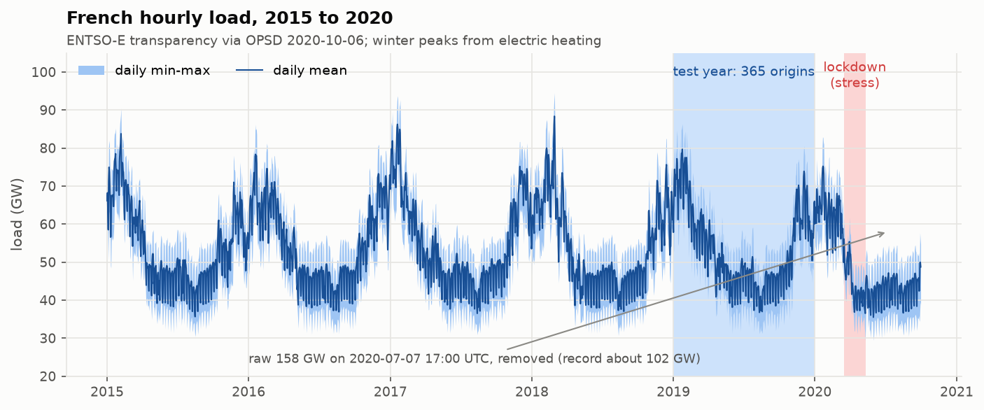
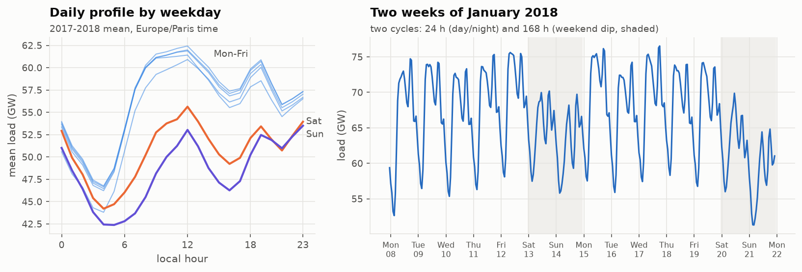
National load is a sum of millions of consumers. It is smooth from hour to hour, it repeats every day and every week, and in France it follows the temperature in winter (electric heating). A good forecaster reads three things: the current level, the daily shape and the weekly shape.
WarningWatch out
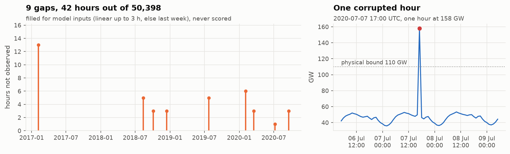
Raw ENTSO-E data contain one hour at 158 GW, against a national record of about 102 GW, and 9 gaps. A single such value in a target window would dominate a mean error. Values outside [20, 110] GW are set to missing. Gaps are filled for inputs only, and an imputed hour is never scored.
2. Choose the baselines honestly
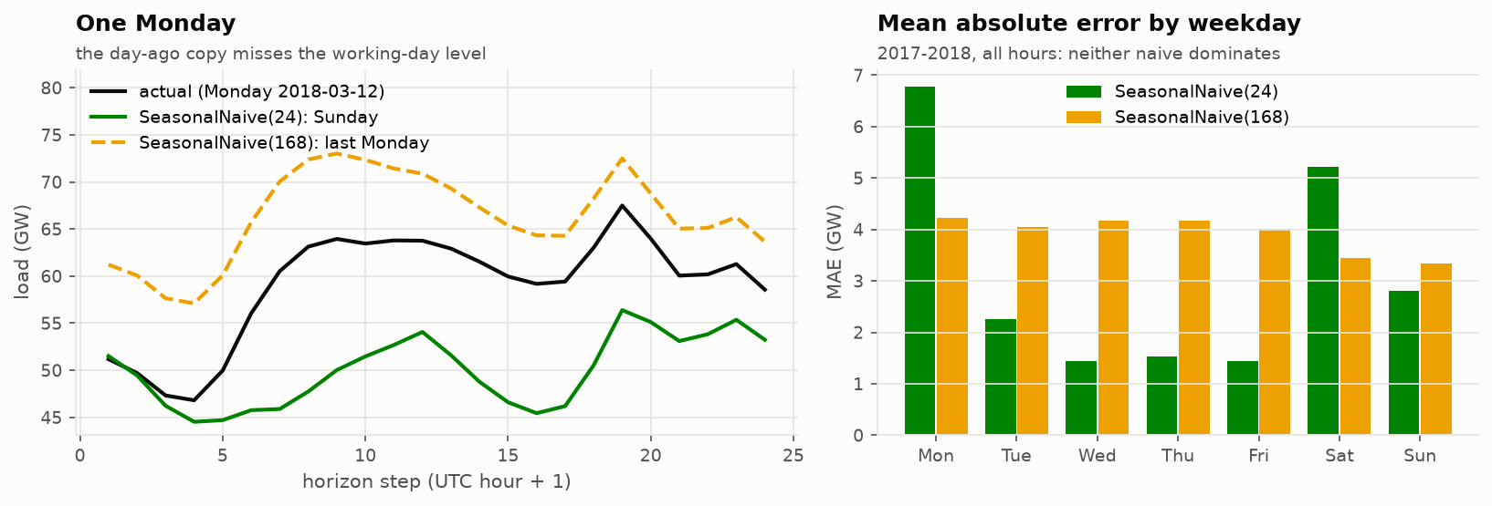
The plan’s naive repeats yesterday, so it forecasts Monday with Sunday. I expected it to be a strawman. The measurement says it beats the weekly naive on five weekdays out of seven, so both stay. The real specialist is MSTL, the only statistical model here that carries both cycles.
3. The protocol: what each model may read
NoteExample
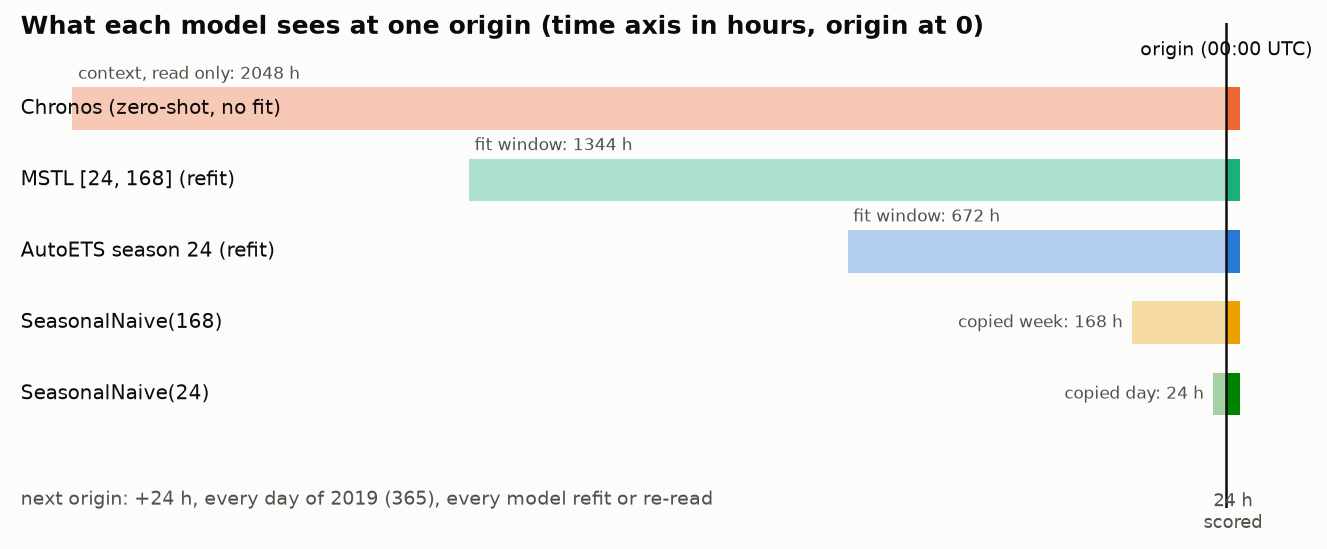
At the origin 2019-03-12 00:00 UTC, AutoETS is refitted on the 672 hours that end at 2019-03-11 23:00. Chronos-Bolt reads the 2048 hours that end at the same hour and is not refitted. Both forecast 2019-03-12 00:00 to 23:00, and the next day the origin moves by 24 hours. tests/test_backtest.py corrupts every value after an origin and checks that its forecast does not move.
The protocol (origins, windows, metrics, verdict rule) was committed before the first forecast. Rule: a challenger beats the reference on a regime if the 95% block-bootstrap CI of its MASE ratio is below 1. It is “deployable as-is” if its 90% coverage is in [0.85, 0.95].
4. The table the plan asks for
sMAPE is utilsforecast’s |e|/(|y|+|f|), half the textbook one. width90 is a fraction of the load. Winkler90 and SQL (scaled quantile loss over 0.1-0.9) are divided by the MASE scale.
WarningWatch out: the reference forecasts a flat line
AutoETS chooses its model by AICc, a one-step likelihood. On smooth hourly data, the level-only model wins at 572 of 608 origins and forecasts 24 times the last value. “Chronos beats AutoETS by a factor 4” is true but says little. A reference with forced seasonality (ETS Z,Z,A) was added after seeing this and is labelled as a deviation. Against it, the factor is 2.5.
WarningWatch out: a flat line can be perfectly calibrated
The flat AutoETS covers 0.899 of hours with its 90% interval, almost exactly nominal, because the interval is 45% of the load wide. Coverage alone rewards a useless interval. The Winkler score, which charges the width, ranks it last.
5. Where does the “90%” interval come from?
ImportantThe trap of the plan, measured
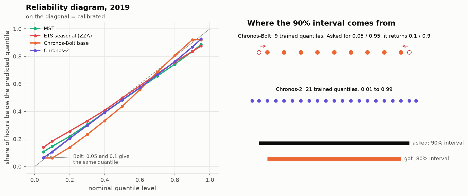
Chronos-Bolt was trained on 9 quantiles, 0.1 to 0.9. Asked for 0.05 and 0.95, it returns its 0.1 and 0.9: its 90% interval is its 80% interval. In the table, cov80 = cov90 = 0.858. It lands inside the band only because its 80% interval over-covers, and the CI of that coverage (0.833-0.884) crosses the band’s edge. The pre-registered rule says WINS; the honest reading is “calibrated by accident”. A split-conformal repair keeps its median and rebuilds the intervals from its own past errors: 0.902.
6. By horizon and by regime
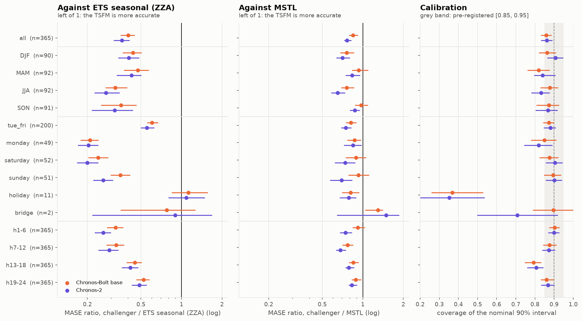
| model | origins | mase_ratio | ratio_lo | ratio_hi | cov90 | verdict |
|---|---|---|---|---|---|---|
| Chronos-Bolt base | 11 | 1.123 | 0.854 | 1.553 | 0.367 | NO DIFFERENCE |
| Chronos-2 | 11 | 1.088 | 0.805 | 1.48 | 0.352 | NO DIFFERENCE |
TipTakeaway: the one sentence of the plan
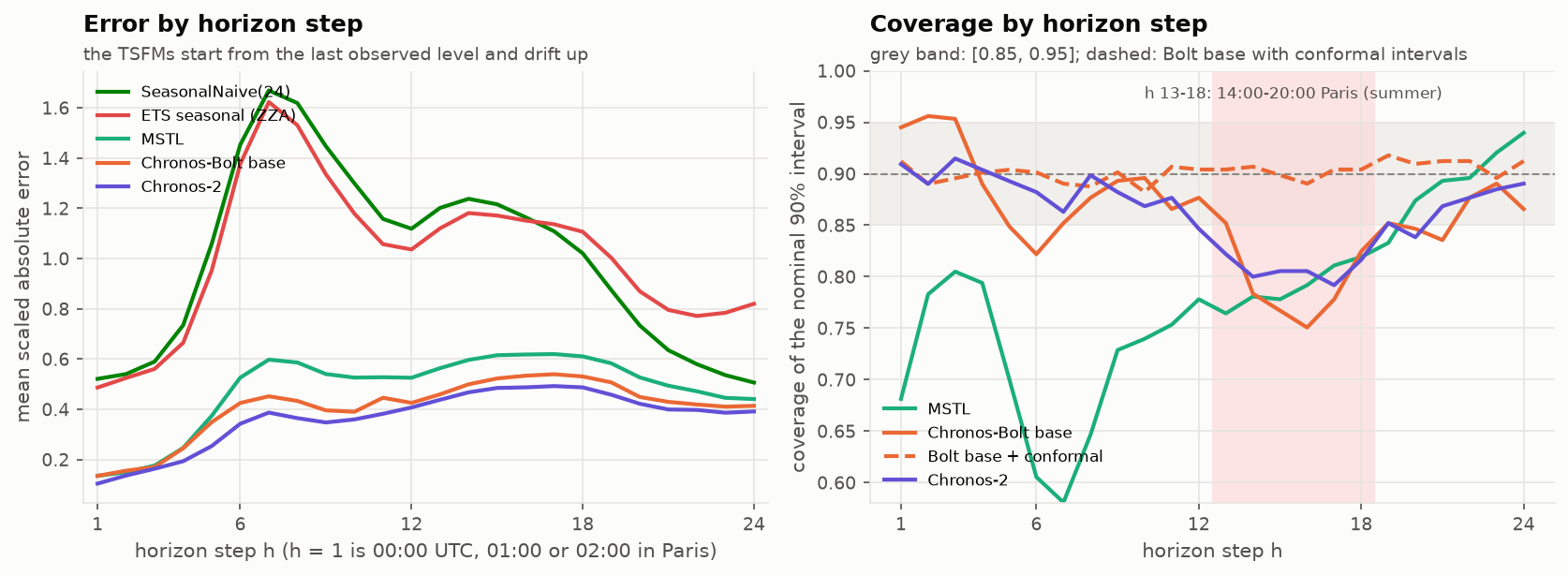
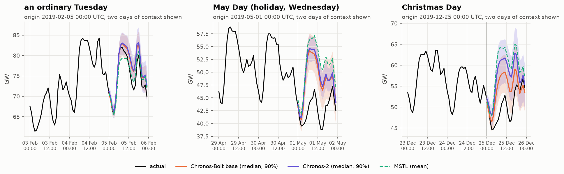
On French hourly load in 2019, Chronos-Bolt base beats AutoETS at every horizon step and on every ordinary day type (MASE ratio 0.24, or 0.40 against a seasonal ETS), with a 90% coverage of 0.86. That interval is its 80% one by construction, and it under-covers on h 13-18 (0.79). On public holidays it is no better than the seasonal ETS and its interval covers 37% of the hours: zero-shot, it does not know the calendar.
The specialists fail on holidays too, but a specialist can be given a holiday flag, while a zero-shot univariate TSFM cannot be told. The conformal repair does not save holidays (0.40), because it calibrates on average over the previous 56 days, not conditionally on a rare day.
Can it be told? (exploratory)
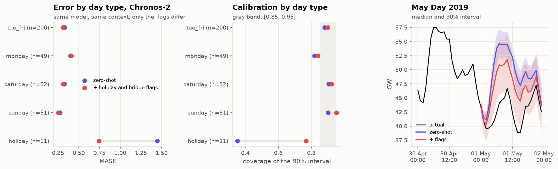
| MASE | cov90 | holidays MASE | holidays cov90 | |
|---|---|---|---|---|
| Chronos-2 zero-shot | 0.365 | 0.862 | 1.446 | 0.352 |
| + holiday and bridge flags | 0.331 | 0.899 | 0.745 | 0.769 |
NoteExploratory, found after the results
Chronos-2 accepts known future covariates. Two 0/1 flags (public holiday, bridge day), known in advance, halve its holiday error (ratio 0.52 [0.39, 0.67]) and bring its yearly 90% coverage to 0.899. Holiday coverage, 0.77 [0.64, 0.89], is below the band as an estimate. “Zero-shot” does not have to mean “blind”: the limit found above is that of a univariate zero-shot model. A pre-registered test on another year should confirm it before any client sees it.
7. Six origins, as in the plan?
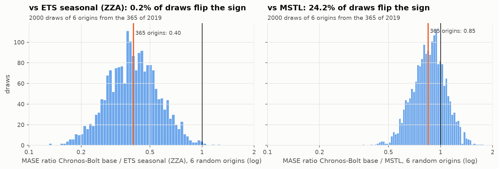
With 6 origins drawn at random, the comparison against the seasonal ETS is right 99.8% of the time, since the gap is a factor 2.5. Against MSTL, the close contest, a quarter of the draws reverse it. The minimum of the plan detects large gaps and cannot settle close ones.
8. Stress and sensitivity
NoteExploratory, not pre-registered
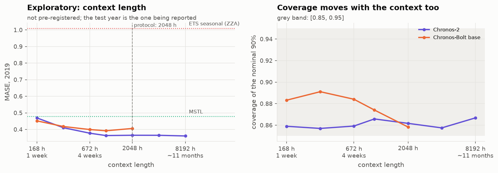
With one week of context, Bolt base (0.452) already beats MSTL fitted on eight weeks (0.479). That is the cold-start argument the router of block 3 tests across 50 series. The best context on 2019 (1024 h) is not adopted, because it was found on the test year.