4 · Reading: the MASE
Hyndman & Koehler (2006), FPP3 section 5.8, shown on figures
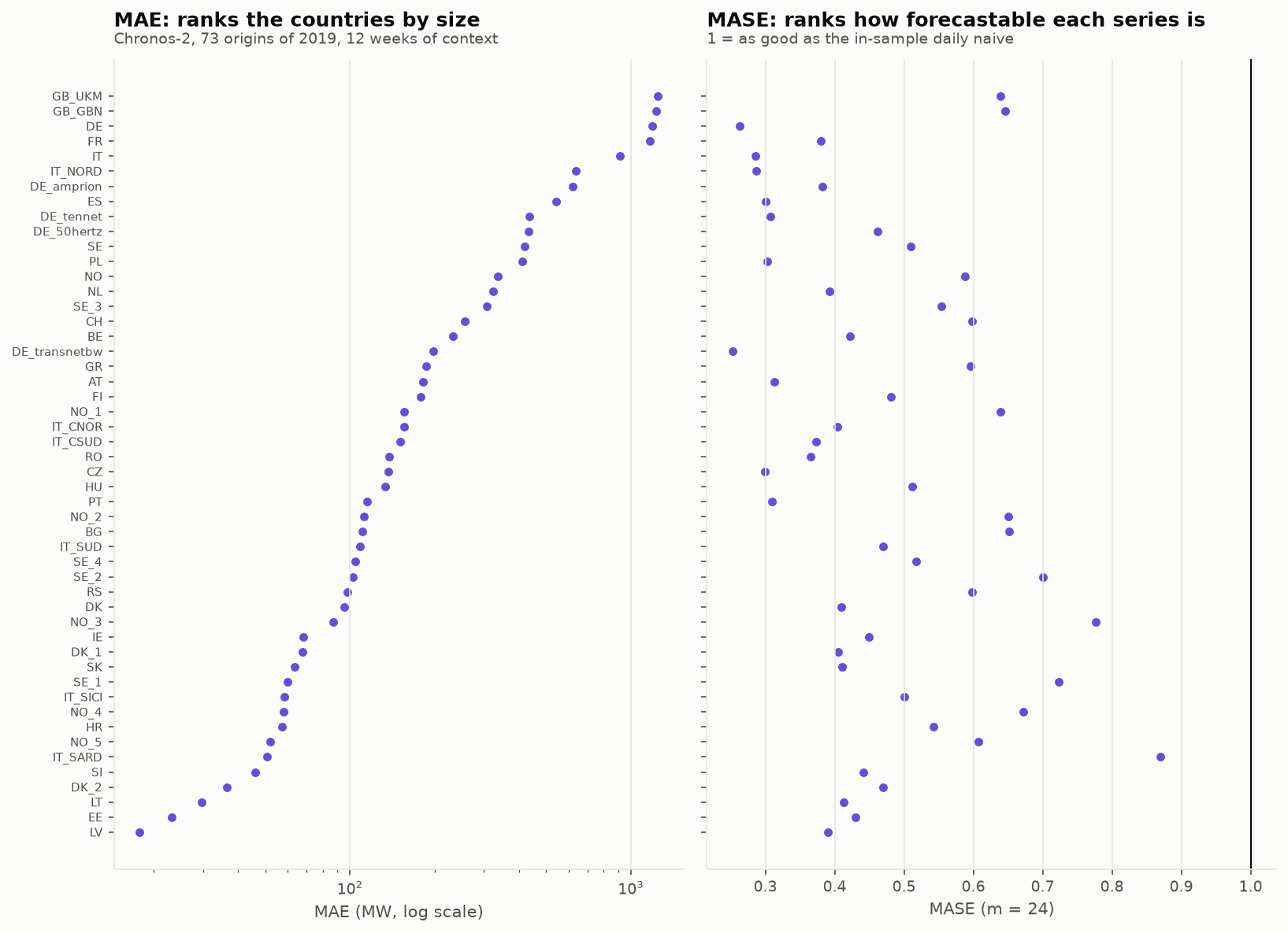
An error of 1,000 MW is large for Belgium and small for Germany. A percentage fixes that, but it breaks near zero. The MASE divides the error by the error a naive method made on the same series in the past. It answers “how much better than doing nothing clever?”, in a unit that is the same for every series.
\[ \text{MASE} = \frac{\frac{1}{h}\sum_{j=1}^{h} |y_{T+j} - \hat y_{T+j}|}{\frac{1}{T-m}\sum_{t=m+1}^{T} |y_t - y_{t-m}|} \]
The 2006 paper defines it with m = 1 (one-step naive). The seasonal version with lag m is FPP3 section 5.8. This study uses m = 24.
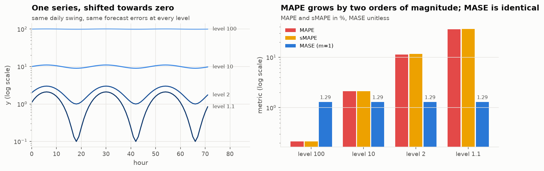
Why not MAPE
Why not sMAPE either
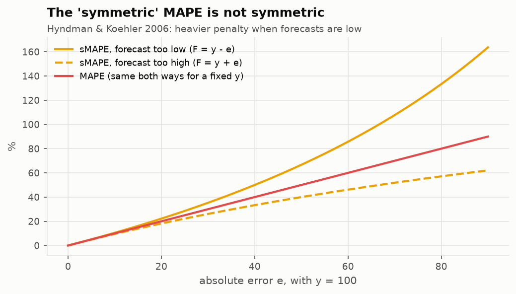
For y = 100 and an error of 60, sMAPE gives 86% if the forecast is low and 46% if it is high. A model that over-forecasts looks better. utilsforecast’s smape is moreover half the textbook formula.
What scale-free buys
The scale is a choice
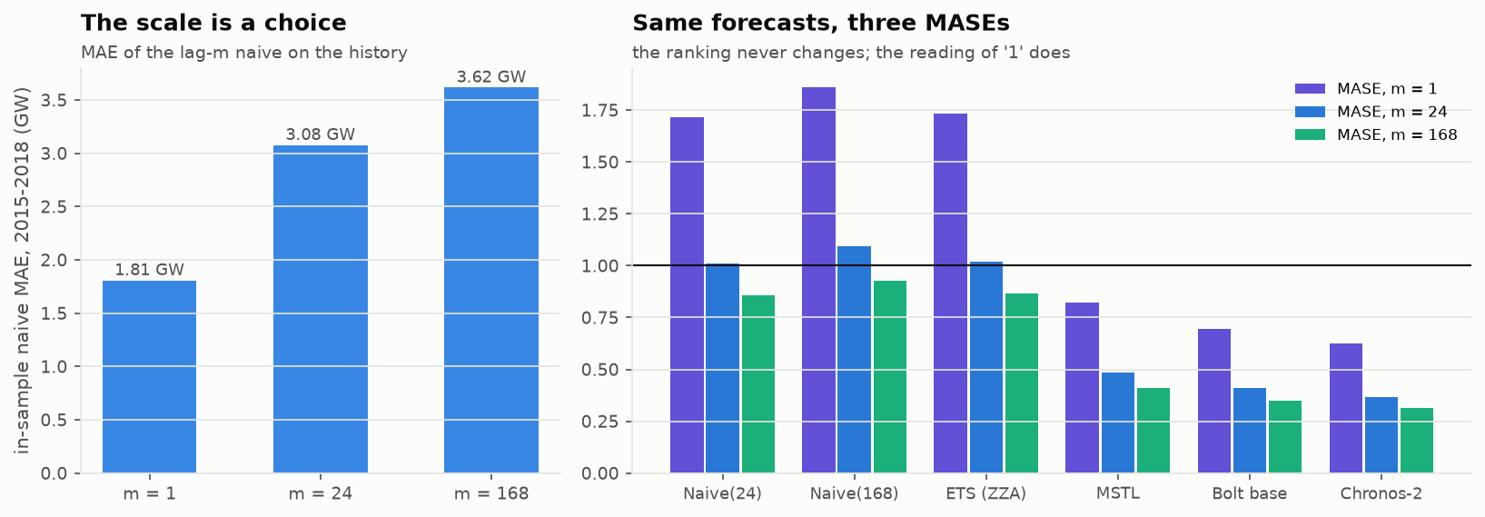
With m = 24, SeasonalNaive(24) scores 1.01: out of sample it repeats the method that defines the scale. With m = 1, the same forecasts score 1.72. “MASE below 1” only means something once m and the horizon are stated.